
The story
I wanted to see whether training a small Transformer on simulated companies would help it make better forecasts from real SEC filings.
After the market crash in spring 2025, I read quarterly reports and came across Jane Street’s Real-Time Market Data Forecasting competition on Kaggle. People there were building models to forecast markets, and I wanted to build one too. At the time I did not have the technical knowledge for it. When I later read the Q2 2026 reports, I remembered the idea. By then, projects such as the GPT-2 piano, LocalSR and Nature Inventory Delta had given me a broad idea of how I could approach the problem.
The implementation
The dataset contains 11,569 quarterly and annual reports from 305 US industrial companies from 2010 to 2026, all taken from the SEC’s EDGAR database. The model doesn’t try to predict the stock price years from now. It forecasts how far the stock can move relative to the industrial sector fund (XLI) over the next 5 and 20 trading days. The clock starts at the first market open at least 30 minutes after the SEC accepted the report as this is when people can start to act on it.
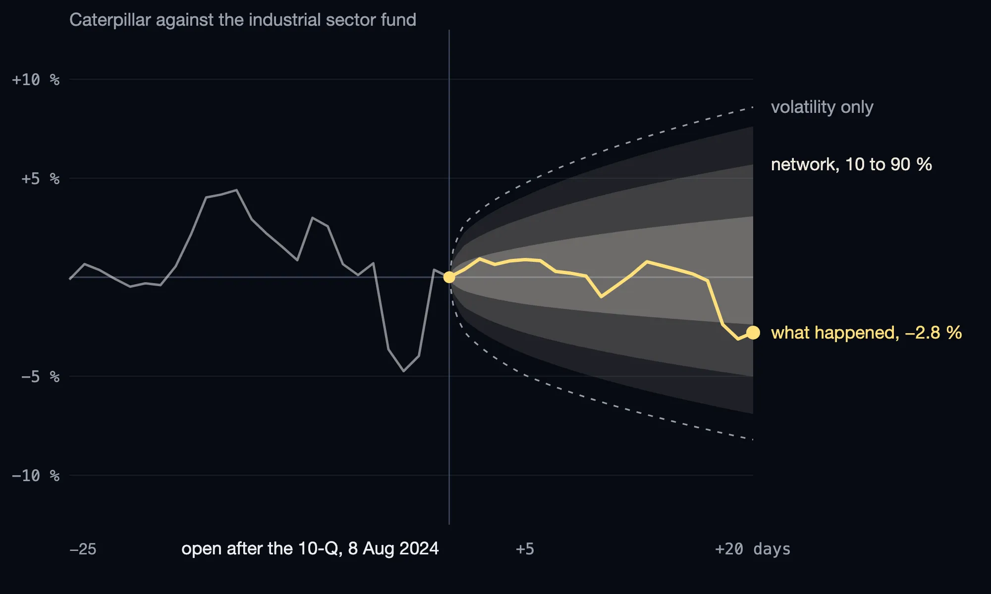
I first trained the model on simulated companies with invented reporting habits and then on the real filings before 2022, and kept 2022 for validation. Before the final test, I wrote the rules down and saved a checksum of them, and the code refuses to compute any result if that file changes. I compared it with four baselines: a forecast based on the stock’s recent volatility, a linear model, boosted trees, and the same network without the simulator.
The results
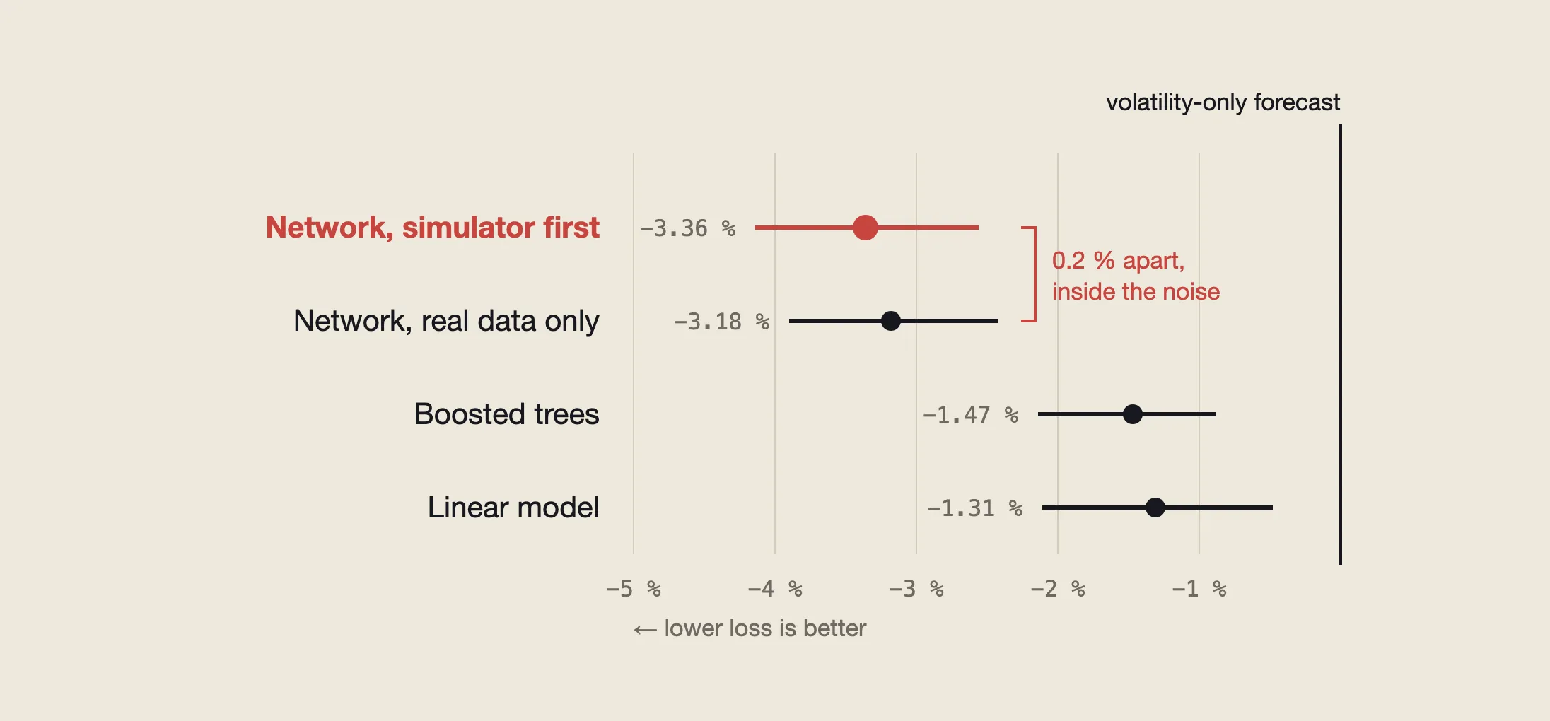
In the final test (3,329 filings from 2023 to 2026), the network’s loss was 3.4 % lower than the volatility forecast, 2.1 % lower than the linear model and 1.9 % lower than the boosted trees. That held in all three runs and even on 867 filings from companies it had never seen. The simulator did not make a clear difference. The same network trained only on real filings was 0.2 % behind, which is inside the noise.
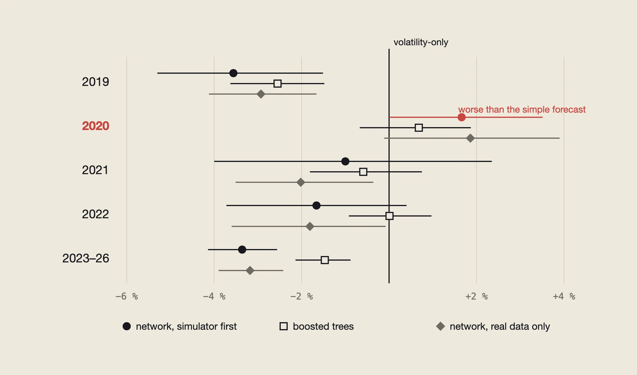
What the network doesn’t know is which way a stock goes. Every model was right about 50 % of the time, and always guessing “down” got 54.4 %. So the improvement is in the width of the forecast ranges. It also didn’t hold every year: in 2019 the network was 3.6 % better than the volatility forecast, and in 2020 it was 1.7 % worse. And that volatility forecast is a simple one. The trees did as well without the filings as with them, and the part of the network meant to remember corrections did nothing, not even in simulation.
Technical details
The network is a pre-norm Transformer encoder with 6 layers, width 256, 8 attention heads and no dropout, 5,140,487 parameters in total. It reads three kinds of tokens. A fact token is one of up to 128 revenue or inventory records, which a linear layer and a GRU cell build from 10 numbers: the year-over-year growth, which metric it is, its version, whether it is a revision, how old the period and the record are, and how late it was reported. A market token is one of 96 trading days and holds the excess return against XLI, its absolute value, the position in the window, and how many earnings releases and filings came out that day. At the end, three learned query tokens, one per horizon (1, 5 and 20 sessions), collect the answer.
Each query outputs seven quantiles (5, 10, 25, 50, 75, 90 and 95 %). They can’t cross, because the model only predicts the median and positive steps outwards (a softplus, summed up), which are in units per square root of a session and then get scaled by √h. The loss is the pinball loss over the seven quantiles, divided by √h, so the 20-day horizon doesn’t dominate.
Pretraining ran on 300 million tokens of simulated companies (20,650 steps, batch 64, AdamW at 5e-4, bf16 on an RX 9060 XT). Every simulated company has an economic process, a disclosure process that decides when numbers come out, how late and how often they get revised, and a market that reacts to it. In 40 % of these worlds the filings say nothing about future returns, so the model learns not to invent a signal where there is none. Fine-tuning on the real filings used AdamW at 2e-4 with cosine decay, at most 15 epochs and early stopping on 2022.
The volatility forecast scales the last 20 days’ volatility by √h and takes its quantiles from the training data. The linear model is one quantile regression per quantile and horizon, and the trees are gradient-boosted quantile models on hand-built features with the same information. Between training and test there is a gap of 20 + 5 sessions, so no label can leak, and the confidence intervals come from 2,000 bootstrap resamples of whole weeks.
The numbers come from the SEC’s XBRL data with every version kept, so the model only sees a value the way it was known on that day. The filing times come from the SEC’s XBRL archive and the filing pages, because the bulk download has the wrong time for about two thirds of the filings. Prices are from Yahoo.